Graphing Exercise Part 3:
Step-by-step instructions for Graphing with Microsoft Excel®
1. Prepare a formatted diskette for saving your work. Remember to save your work periodically throughout this exercise.
2. Double click the Microsoft Excel® icon on the Desktop or Microsoft Office Toolbar with the mouse. (If no icon is shown, click: Start, then highlight Programs-Microsoft Office-Microsoft Excel, and then click the left mouse button.) The Excel program should now be running, and you have a blank Excel Worksheet “Sheet 1” on the screen.
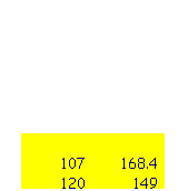
3. Input the set of data assigned to you in the upper right corner of Sheet 1 to make a data table similar to the one shown on the left below: (This set of data is taken from Graphing Worksheet, Part 1.)
|
(Your Name) |
X |
Y |
|
|
|
107 |
168.4 |
|
|
|
120 |
149 |
|
|
|
136 |
126.7 |
|
|
|
150 |
109.5 |
|
|
|
161 |
98.9 |
|
|
|
183 |
67.7 |
|
|
|
191 |
57.4 |
|
|
|
212 |
27.7 |
|
4. Highlight the data values and the headings, X and Y, as shown on the right above.
5.
Click the Chart Wizard button (![]() )
on the menu bar.
)
on the menu bar.
6. Select XY(Scatter) under Chart type. Click the graph style in the upper left corner (only dots, no connecting lines). Click NEXT> to continue or Cancel to start over.
7. In the next step of Chart Wizard, you should find the correct data locations in the Data range entry and, under Series in, Columns is selected. Click NEXT> to continue or Cancel to start over.
8. In the 3rd step of Chart Wizard, you may add/delete the following by clicking respective Tabs:
Type in “Data Set 1 (YOUR NAME)” as the Title for your graph using the Title Tab
Add (or delete) gridlines on the graph using the Gridline Tab
Remove the legend box using the Legend Tab
Click NEXT> to continue or Cancel to start over.
9. In the last step of Chart Wizard, select As object in to place the scatter plot in the current sheet.
10. Click Finish and the scatter plot should be displayed on sheet 1, next to the data table.
11. More likely than not at this point, your plot needs to be re-scaled. For detailed instructions to move, re-size, and edit your plot, refer to the scale and How do I edit my graph sections of this web site: http://www.ksu.edu/stats/tch/malone/computers/excel/
12. Add a best-fit line to your graph as follows: Click anywhere in the scatter plot, chose Chart on the menu bar, and then select add trendline.
13. From the add trendline menu, choose
Linear under the Type Tab; and Display equation on Chart & Display R-square value on Chart under the Options Tab.
Press OK.
14. A straight line calculated by the least-square fit method should appear on your scatter plot, along with its equation and R-square value. To display the equation clearly, you may need to move the textbox to a better location in the chart area.
15. After you have adjusted your scatter plot as desired, click any blank cell in Sheet 1 and select Print Preview under File in the menu bar.
16. Based on what you see in the print preview, select in the print setup menu to landscape so that print preview shows the data table with your name and the scatter plot both in one printed page.
17. Press Print and obtain a hardcopy,
18. Interpolate your scatter plot to obtain the value of Y for a given X and the value of X for a given Y as indicated in the data set assigned to you. For each interpolation, show work on your hardcopy by drawing 2 lines that meet each other at the best-fit line as shown in Figure 1(b).
19. Submit this hardcopy as your report for Part 3.